OWS Styling HOW-TO Guide: Components
Simple Linear Components
Now lets return to the configuration from the worked example in the introduction and look at it in a bit more detail:
rgb_cfg = {
    "components": {
        "red": {"red": 1.0},
        "green": {"green": 1.0},
        "blue": {"blue": 1.0},
    },
    "scale_range": (50, 3000),
}
The components section lets you specify the three output image RGB channels independently.
It is important not to get confused between the keys of the outer dictionary, which are the output image channels and should always be “red”, “green” and “blue”; and the keys of the inner dictionaries, which are measurement bands of the ODC data being styled.
It’s easiest to explain with some examples. We will use the same test data as in the introduction, but this time we will select all the available measurement bands, so we can re-use the same data for all the examples in this section.
from datacube import Datacube
dc = Datacube()
data = dc.load(
    product='ls8_nbart_geomedian_annual',
    measurements=['red', 'green', 'blue', 'nir', 'swir1', 'swir2'],
    latitude=(-16.1144, -13.4938),
    longitude=(140.7184, 145.6924),
    time=('2019-01', '2019-01'),
    output_crs="EPSG:3577",
    resolution=(-300,300)
)
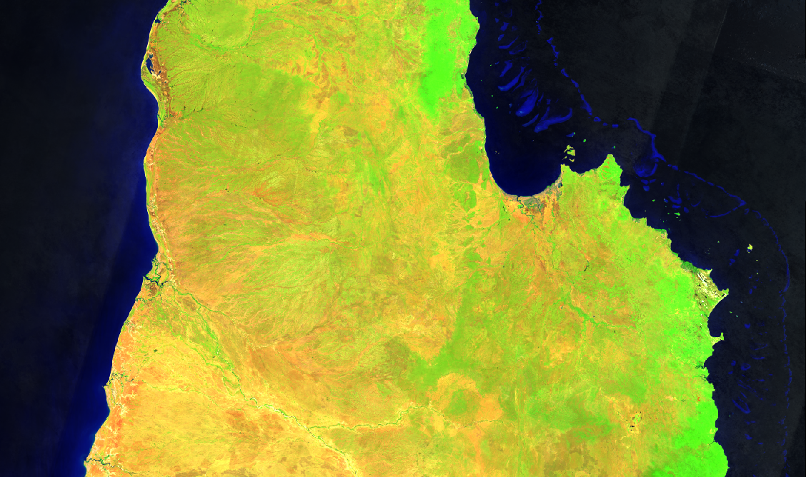
Example: Infrared/Green False Colour
Lets start with a popular false-colour style, using optical green and two infrared bands. Note that the “green” band of the data is not assigned to the “green” channel of the output image.
ir_green_cfg = {
    "components": {
        "red": {
            "swir1": 1.0
        },
        "green": {
            "nir": 1.0
        },
        "blue": {
            "green": 1.0
        },
    },
    "scale_range": (50, 3000),
}
Example: Greyscale single band
If we wanted a greyscale image of a single band (say red), you could do this:
pure_red_cfg = {
    "components": {
        "red": {
         "red": 1.0
        },
        "green": {
         "red": 1.0
        },
        "blue": {
         "red": 1.0
        },
    },
    "scale_range": (50, 3000),
}
Example: Mixing bands
What if we want to mix more than one band to make each channel? We can simply add more bands to the various colour channel dictionaries, with multiplying factors. Normally we ensure that the multiplying factors for each channel sum to 1.0, so the result is a (possibly weighted) average of the input bands, but this is not enforced.
Here we average all three visible bands into the red channel, put near infra-red in the green channel and average the two shortwave infrared bands to make the blue channel:
all_bands_cfg = {
    "components": {
        "red": {
            # Weighting factors should sum to (close to) 1.0
            # 0.333 + 0.333 + 0.333 = 0.999 ~ 1.0
            "red": 0.333,
            "green": 0.333,
            "blue": 0.333,
        },
        "green": {
            # Weighting factors should sum to (close to) 1.0
            # So use 1.0 for a single band.
            "nir": 1.0
        },
        "blue": {
            # Weighting factors should sum to (close to) 1.0
            # 0.5 + 0.5 = 1.0
            "swir1": 0.5,
            "swir2": 0.5,
        },
    },
    "scale_range": (50, 3000),
}
Example: Unused channels
If you don’t want to write any data to one or more of the image channels (red, green or blue) just leave it empty:
only_red_cfg = {
    "components": {
        "red": {
            "red": 1.0
        },
        "green": {},
        "blue": {},
    },
    "scale_range": (50, 3000),
}
Scale Ranges: Controlling dynamic range
What about the other part of that config - the scale_range part? The scale range specifices the value
range of the input data that will be mapped to the output channel range (0-255).
Let’s try some other values and see what happens.
Firstly, let’s remind ourselves of our original RGB configuration and image:
rgb_cfg = {
    "components": {
        "red": {"red": 1.0},
        "green": {"green": 1.0},
        "blue": {"blue": 1.0},
    },
    "scale_range": (50, 3000),
}
In this image, band values between 50 and 3000 get scaled to the image values 0 to 255. (Values less than zero are clipped to 0 and values greater than 3000 are clipped to 255.)
Example: Low Scale Range
Let’s start by pulling the scale_range down a bit:
rgb_low_scale_rng_cfg = {
    "components": {
        "red": {"red": 1.0},
        "green": {"green": 1.0},
        "blue": {"blue": 1.0},
    },
    "scale_range": (10, 800),
}
As you can see, the resulting image looks saturated, washed out and overly bright. So if your first guess at scale_range values produced an image like this, you probably want to increase your scale_range a bit.
Example: High Scale Range
rgb_high_scale_rng_cfg = {
    "components": {
        "red": {"red": 1.0},
        "green": {"green": 1.0},
        "blue": {"blue": 1.0},
    },
    "scale_range": (1000, 8000),
}
Whoops too far! Now it’s almost pure black! If your image looks like this, you need to pull your scale_range down:
Example: Narrow Scale Range
rgb_narrow_scale_rng_cfg = {
    "components": {
        "red": {"red": 1.0},
        "green": {"green": 1.0},
        "blue": {"blue": 1.0},
    },
    "scale_range": (1000, 3000),
}
This is getting better, the brightest parts are nice and bright, but the lower end of the scale range is too high,
leaving too much image clipped to black. If you keep adjusting back and forth,
you’ll eventually end up more or less where we started, with a scale_range around (50,3000).
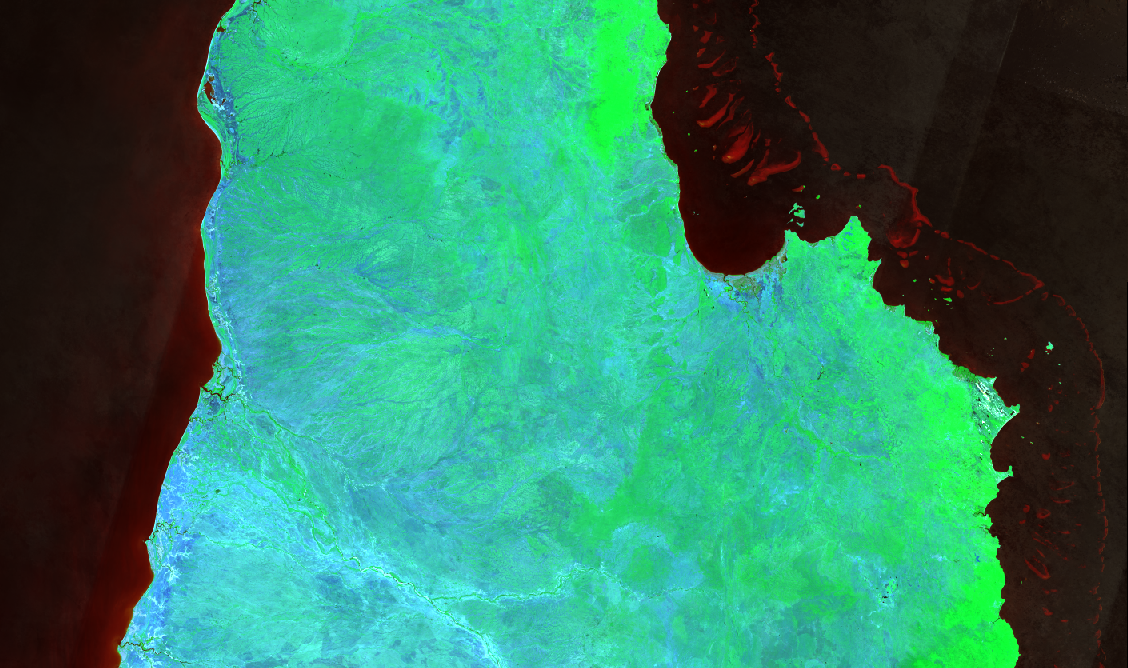
Example: Per-channel scale_ranges
What if we want to apply different scale ranges to different channels?
For example, the image in the false colour example above, looks a bit saturated, especially in the red and green channels (red+green makes yellow).
Let’s see what we can do with some judicious tweaking of the scale_ranges on a per-band basis:
irg_bandscale_cfg = {
    "components": {
        "red": {
            "swir1": 1.0,
            "scale_range": (1500, 3700),
        },
        "green": {
            "nir": 1.0,
            "scale_range": (1600, 3200),
        },
        "blue": {
            "green": 1.0
        },
    },
    "scale_range": (200, 1900),
}
The red and green channel have custom scale ranges.
The “blue” channel does not have a custom scale_range, so it takes the default scale_range (200,1900).
(The default scale_range may be omitted where it is not needed.)
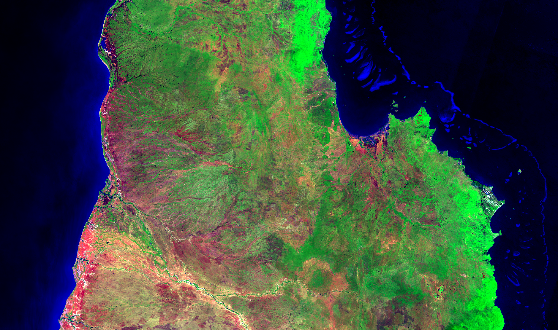
Wow! That looks much better!
But don’t get too carried away! You’ll probably find that these particular scale range values look really dark and washed out in south eastern australia, or super bright and saturated in the central deserts. The trick is usually to choose a few datasets from different land cover types across the whole area covered by the data, and come up with a compromise configuration that looks reasonably good everywhere.
But as any scientist will tell you, when it comes to visualisation, linear equations can only get you so far, so next we start to look at how to apply more powerful maths to calculate components.