OWS Styling HOW-TO Guide

Table of Contents

• OWS Styling HOW-TO Guide

  • Introduction

    • Scope

    • Introduction - Testing styles

Introduction

Scope

This HOW-TO Guide is aimed at scientific staff with a good understanding of their data product and the use of the Open Data Cube (ODC). It aims to:

1. provide some specific examples of how to call the OWS Styling API to generate test images from raw ODC data.

2. demonstrate how to configure OWS styles with real-world examples.

For thorough technical description of the configuration format, see the configuration documentation.

Setting up an ODC environment and installing datacube-ows is also beyond the scope of this HOWTO, but if you are using a JupyterHubs based system like DEA Sandbox, a Quick Start Guide is available.

Introduction - Testing styles

We’ll start with a quick but complete walk through the process of creating an image with the API.

First of all, you’ll need some data. Select a bounding box (in lat/long), a date, a resolution, and an output CRS, the measurement bands you need, and obtain your data from the Open Data Cube.

Note that it is essential that you select all the bands used by your style definition.

from datacube import Datacube
dc = Datacube()
data = dc.load(
    product='ga_ls8c_nbart_gm_cyear_3',
    measurements=['red', 'green', 'blue'],
    latitude=(-16.1144, -13.4938),
    longitude=(140.7184, 145.6924),
    time=('2019-01', '2019-01'),
    group_by='time',
    output_crs="EPSG:3577",
    resolution=(-300,300)
)

Note

If apply_ows_style_cfg() returns

WMSException: Style stand_alone does not support requests with 2 dates

set group_by='solar_day'

This query results in an xarray dataset, and therefore a final image, with a pixel resolution of 1128x668.

Now we create a style configuration dictionary. We’ll start with a simple RGB “true colour” visualisation.

rgb_cfg = {
    "components": {
        "red": {"red": 1.0},
        "green": {"green": 1.0},
        "blue": {"blue": 1.0},
    },
    "scale_range": (50, 3000),
}

Don’t worry yet about understanding what that all means, we’ll cover that later. For now, we can apply this style to the data, and write the result to disk as a PNG file:

from datacube_ows.styles.api import StandaloneStyle, apply_ows_style_cfg, xarray_image_as_png

xr_image = apply_ows_style_cfg(rgb_cfg, data)
png_image = xarray_image_as_png(xr_image)
with open("example1.png", "wb") as fp:
     fp.write(png_image)

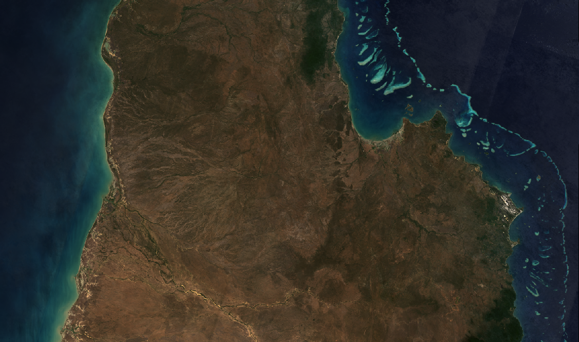
The resulting image looks like this:

If you are using a notebooks based environment like JupyterHub, you can display the image using the plot_image API functions:

# Assumes the spatial dimensions are called "x" and "y".
plot_image_with_style_cfg(rgb_cfg, data)

# If the spatial dimensions have other names, you must pass them in manually, e.g.:
plot_image_with_style_cfg(rgb_cfg, data, x="longitude", y="latitude")

View full size

Refer to the documentation for more information about the OWS styling API.

Next we start to look at how style configurations work.